Rendering Fractals by Optimizing Pixels in JAX
Update (2025-07-25)
I’ve ported this to CUDA and made it much faster. Check it out here.

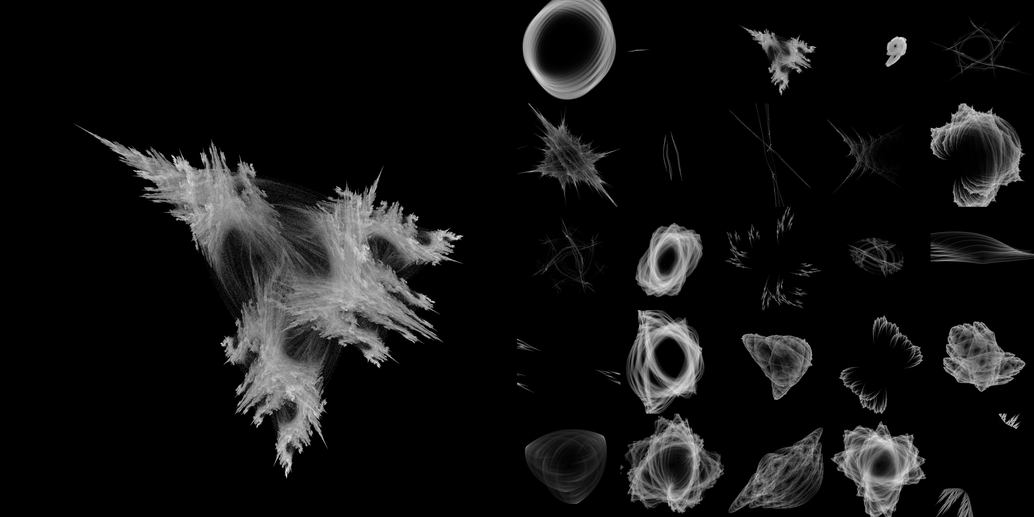
Some Fractals I Generated
Introduction
I’ve been fascinated by fractals from a young age and how simple rules can generate complex patterns. In this post, I’ll be going over how I used the machine learning library JAX to quickly render fractals.
Why JAX?
JAX makes it easy to write performant parallel code that can run on CPUs, GPUs, TPUs, and other accelerators. It uses XLA to compile the code to run on device, and it has a JIT compiler that can optimize your code’s execution. Writing JAX code is very similar to writing NumPy code, since JAX includes many of the same APIs.
Iterated Function Systems
The type of fractal I’ll be rendering is an Iterated Function System. An Iterated Function System is a collection of functions that are repeatedly applied to a starting point. By iteratively applying these functions to the starting point and tracking the result points, we can generate a fractal. Calculating the result of applying every combination of the functions to the starting point is computationally expensive, so I chose to use a fixed number of points and randomly choose which function to apply to each point, instead of applying every function to every point.
Chosen Transformations
I used a system of two functions, and chose to use the origin as the starting point. The functions I used were of the form of a composition of:
- A matrix multiplication
- A vector addition
- A scalar multiplication by a power of the distance from the origin
In math, this looks like:
Applying Transformations
In JAX, applying this class of transformation to a list of points looks like this:
def apply_transform(x, y, settings):
    a, b, c, d, e, f, power = settings

    x_prime = x * a + y * b + c
    y_prime = x * d + y * e + f

    scale_squared = x_prime ** 2 + y_prime ** 2
    # divide by 2 for square root
    x_prime /= scale_squared ** (power / 2)
    y_prime /= scale_squared ** (power / 2)

    return x_prime, y_prime
Updating Points
The following function randomly applies one of the transforms to the points to get the next set of points. This is similar to the Chaos Game method.
import jax
import jax.numpy as jnp

dtype = jnp.float32

def update(x, y, settings, rng):
    rate, settings_1, settings_2 = settings

    # apply the first transform to the points
    x_prime_1, y_prime_1 = apply_transform(x, y, settings_1)
    # apply the second transform to the points
    x_prime_2, y_prime_2 = apply_transform(x, y, settings_2)

    # randomly choose one of the transforms (chaos game)
    mask = jax.random.uniform(rng, shape=(x.shape[0],), minval=0, maxval=1, dtype=dtype)
    mask = 1 * (mask < rate)

    # choose the first transform where the mask is 1
    # and the second transform where the mask is 0
    x = x_prime_1 * mask + x_prime_2 * (1 - mask)
    y = y_prime_1 * mask + y_prime_2 * (1 - mask)

    return x, y
Parallelism
It’s important to note that the code transforms many points at once. This allows the program to generate images more quickly on most modern hardware. The points will all start at the same position, but will diverge as different transforms are randomly chosen.
Optimizing Pixels
Let’s refer to the rate at which the points appear within a pixel as the “density” at that pixel. To generate an image, we can treat lower density pixels as black and higher density pixels as white. To go from transforming points to generating an image of a fractal, we can start with a black image (zero density) and iteratively update the pixels based on the current set of points.
We can use an optimizer designed for gradient descent to optimize the pixels. Even though we are not using gradient descent (we have no loss function), we can still use the same optimizer while treating the gradient as an update to the density, rather than a set of derivatives of a loss function. We can set the “gradient” to 1 at the current locations of the points and 0 elsewhere to maximize the density at the current locations. I used the PSGD optimizer to optimize the pixels, since it gave the best results for my use case.
import tqdm
import optax
# the optimizer that I found to work the best
from psgd_jax.affine import scale_by_affine

index_dtype = jnp.int32

# density is the vector of the density values at each point
# it is initialized to zeros
# it is updated where the current points are
def optimize(density, batch_size, x_res, y_res, settings, iterations, bounds, rng):
    min_x, max_x, min_y, max_y = bounds

    # use a warmup schedule to start the optimization at a lower learning rate
    schedule = optax.schedules.warmup_constant_schedule(0, 1, iterations // 10)
    optimizer = optax.chain(
        scale_by_affine(), # optimizer
        optax.scale_by_schedule(schedule) # learning rate schedule
    )
    opt_state = optimizer.init(density)

    # start at the origin
    x = jnp.zeros(batch_size, dtype=dtype)
    y = jnp.zeros(batch_size, dtype=dtype)

    # calculate how large each pixel is
    dx = (max_x - min_x) / (x_res - 1)
    dy = (max_y - min_y) / (y_res - 1)

    @jax.jit
    def step(density, x, y, opt_state, rng):
        update_rng, rng = jax.random.split(rng, 2)

        # update the points
        x, y = update(x, y, settings, update_rng)

        # find the nearest pixel to the current points
        x_index = jnp.round((x - min_x) / dx).astype(index_dtype)
        y_index = jnp.round((y - min_y) / dy).astype(index_dtype)

        # go to an invalid index after the end of our vector if the coordinate is negative or too large
        x_index = x_index + (-x_index + x_res) * ((x_index < 0) + (x_index >= x_res))
        y_index = y_index + (-y_index + y_res * x_res) * ((y_index < 0) + (y_index >= y_res))

        # set the gradient to 0 by default
        grad = jnp.zeros((x_res * y_res,), dtype=dtype)
        # set the gradient to 1 at the current locations
        grad = grad.at[x_index * y_res + y_index].set(1)
        # normalize the gradient to help the optimizer converge faster
        grad = jax.nn.standardize(grad, axis=0)

        updates, opt_state = optimizer.update(grad, opt_state, density)
        density = optax.apply_updates(density, updates)

        return density, x, y, opt_state, rng

    # run the optimization for the specified number of iterations
    for _ in tqdm(range(iterations)):
        density, x, y, opt_state, rng = step(density, x, y, opt_state, rng)

    return density
Results
The optimization ran very quickly, at over 1000 optimization steps per second on a T4 GPU with a batch size of 1024 and a resolution of 1024x1024. Since I ran 10000 steps per image, it took less than 10 seconds to generate each image.
I found a somewhat good range of transformation parameters to use that are included in the code, and I would recommend trying to change them to see what kind of results you get.
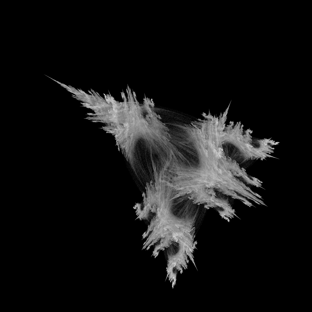
My favorite image of the 25 images I generated is below:

Conclusion
I think this is a pretty cool way to render fractals and a cool use case for JAX. I’m excited to see other ways people use JAX that I haven’t thought of. I hope you find this useful or inspiring!